Increase in Precipitation Efficiency With Surface Warming in Radiative-Convective Equilibrium
Abstract
The precipitation efficiency of convection (ε) plays an important role in simple models of the tropical atmosphere as well as in global climate models' projections of future climate changes, but remains poorly understood and poorly constrained. A particularly urgent question is how ε will change in warmer climates. To address these issues, this study investigates the precipitation efficiency in simulations of radiative-convective equilibrium with a cloud-resolving model forced by a wide range of sea surface temperatures (SSTs). Two different domains are considered: a small, doubly periodic domain, and a 2-D (x-z) “mock-Walker” domain with a sinusoidal SST profile that resembles the equatorial Pacific, and the sensitivities of the results to the microphysical scheme and to the horizontal resolution are also explored. It is found that ε generally increases with warming in the small domain simulations because of increases in the efficiency with which cloud condensate is converted into precipitation, with changes in the re-evaporation of falling precipitation playing a secondary role. This picture is complicated in the 2-D simulations by substantial changes in the degree of convective organization as the underlying SSTs are varied. ε is found to decrease as convection becomes more organized, because convective organization results in relatively more low clouds, which have small (≤0.1) precipitation efficiencies, and relatively less high clouds, which have larger (∼0.4) precipitation efficiencies.
Key Points
- Precipitation efficiency is investigated in RCE simulations with a CRM forced by a wide range of SSTs
- Precipitation efficiency generally increases with warming because of increased cloud density
- Changes in the large-scale circulation can cause precipitation efficiency to decrease
Plain Language Summary
The precipitation efficiency of convection (ε) quantifies the fraction of water that condenses in a cloud that reaches the surface as precipitation. Recent work has shown that changes in ε can play an important role in determining the warming of climate models in response to increases in atmospheric carbon dioxide concentrations, and ε is also a key factor in theories for the dynamics of the tropical atmosphere. Despite this importance, however, ε is poorly understood and poorly constrained. In this study, we take a first step to addressing this issue by investigating how precipitation efficiency behaves in idealized simulations of the tropical atmosphere, in which the underlying sea surface temperature is varied across a wide range of values. We find that ε generally increases with warming because clouds become denser and so form precipitation more easily, though in some cases ε decreases because of changes in the large-scale flow of the tropical atmosphere.
1 Introduction
The precipitation efficiency of convection is a measure of how much of the water that condenses in a rising column of air reaches the surface as precipitation, and can be defined as ε = P/C, where P is the surface precipitation rate (with units kg m−2 s−1) and C is the column-integrated condensation rate (also kg m−2 s−1). ε can be defined at various temporal and spatial scales (see Sui et al., 2007), and in what follows we primarily focus on the tropical-mean, or bulk, precipitation efficiency. Many factors contribute to the precipitation efficiency, particularly the various microphysical processes responsible for the formation and re-evaporation of precipitation, such as the autoconversion rate and the fall speeds of the hydrometeors, as well as cloud-scale dynamics such as entrainment rates, and we do not currently have a good understanding of what sets ε, nor of how its value will change in future climates.
Despite this uncertainty, precipitation efficiency can be tuned quite precisely in some global climate models (GCMs; Zhao, 2014), and several recent studies have found a strong relationship between climate sensitivity and the response of ε to warming (Mauritsen et al., 2012; Tomassini et al., 2015; Zhao, 2014; Zhao et al., 2016). This correlation is thought to come from the effect of ε on clouds, as models in which the precipitation efficiency decreases in warmer conditions are able to maintain greater amounts of cloud cover and thus have a more negative cloud feedback (Sherwood et al., 2014; Zhao, 2014). Zhao et al. (2016) were able to make a single model's cloud radiative effect span the CMIP5 intermodel range in cloud radiative effect by altering the scheme by which cloud condensate is removed as precipitation, with no discernible impact on the quality of the GCM's representation of the present-day climatology. In addition to this relationship with climate sensitivity, ε is also an important factor in models' projections of future changes in the hydrologic cycle, and influences the rate at which aerosols are removed from the atmosphere (Bailey et al., 2015).
 (1)
(1)Given the impact of precipitation efficiency on future climate projections, the fact that it can be prescribed in GCMs and its importance for our conceptual understanding of the tropical atmosphere, better constraints are needed on its value and on how this value might change in a warmer world. These constraints must be obtained from a combination of focused modelling studies and observations, and would directly inform development of the convective parameterizations used in GCMs. As a first step towards this goal, in this study we have investigated how the precipitation efficiency varies in simulations of radiative-convective equilibrium (RCE) with a cloud-resolving model (CRM) as the underlying sea surface temperature (SST) is varied. We consider both doubly periodic, small domain simulations and 2-D “mock-Walker Cell” simulations, which include horizontal SST gradients and so allow us to investigate how ε is affected by the presence of a large-scale circulation.
 (2)
(2) , εe approaches the ε defined in the first paragraph. Equation 2 suggests that ε should decrease as relative humidity increases, but this is not a very stringent constraint, and applies only when convection behaves as a single entraining plume. In simulations Romps found that ε was sometimes twice as large as the 1 − RH lower bound.
More speculatively, it has been suggested that an increase in convective aggregation with warming could increase precipitation efficiency (Mauritsen & Stevens, 2015). However, past studies have found inconsistent tendencies with warming: In GCMs aggregation has been found to increase with warming (Arnold & Randall, 2015) and to have a nonmonotonic dependence on SST (Coppin & Bony, 2015). Becker et al. (2015) showed that the temperature dependence of aggregation in GCMs is sensitive to the details of the convective parameterization, especially to the entrainment rate. Similarly, CRM studies have found aggregation to increase with SST (Wing & Emanuel, 2014) and to be nearly independent of SST (Cronin & Wing, 2017; Holloway & Woolnough, 2016; Wing & Cronin, 2016). None of these studies have carefully examined the changes in bulk precipitation efficiency resulting from convective aggregation.
In large-eddy simulations of individual cumulus congestus clouds, Langhans et al. (2015) found precipitation efficiencies between 0.3 and 0.4 and demonstrated that the “sedimentation efficiency” (the probability of a falling hydrometeor reaching the surface) is the dominant control on precipitation efficiency in their model. In coarser-resolution simulations of RCE with CRMs, ε is typically found to be between about 0.2 and 0.5 (e.g., Pauluis & Held, 2002b; Romps, 2011; Tao et al., 2004), but no systematic investigation of what sets the value of ε nor of how ε varies with warming has been carried out in models of this type.
Precipitation efficiency is difficult to measure observationally. Lau and Wu (2003) used satellite retrievals of rainfall and cloud liquid water to demonstrate that the precipitation efficiency of warm rain increases as the underlying SST increases, but this result required the use of a microphysical parameterization to convert the satellite data into precipitation efficiencies. Recently, Bailey et al. (2015) used water vapor isotope ratios to measure ε near Hawaii's Big Island and found that synoptic weather plays an important role in setting the precipitation efficiency, with different types of weather systems having very different efficiencies.
None of these studies have provided the parameter dependence of ε needed by GCMs, however, and characterizing the precipitation efficiencies in our CRM simulations is an important intermediate step towards obtaining this goal. With the CRM, we are able to perform a large number of simulations to investigate the sensitivity of ε in our model to the underlying SST, the microphysical scheme, the horizontal grid resolution and the presence of a large-scale circulation. We have also used a similar framework to Langhans et al. (2015) to diagnose the factors which determine ε, providing a physical explanation for why ε varies as it does.
The model, experiments, and diagnostic framework are presented in the next section. The results of the small domain experiments are presented in section 3, and the 2-D mock-Walker simulations are discussed in section 4. We end with a summary and conclusion in section 5.
2 Methods
2.1 Model and Experiments
The cloud-resolving model that we use in this study is version 6.10.8 of the System for Atmospheric Modeling (SAM; Khairoutdinov & Randall, 2003). This model solves the anelastic continuity, momentum, and tracer conservation equations, and its prognostic thermodynamic variables are liquid/ice water static energy, total nonprecipitating water (vapor, cloud water, and cloud ice), and total precipitating water (rain, snow, and graupel).
All simulations were conducted without rotation and with fixed SSTs. The small domain simulations were performed on a square, doubly periodic domain, with width 96 km. As found by Muller and Held (2012), this domain size is small enough to prevent convective self-aggregation. The mock-Walker simulations were performed on a 2-D (x − z) domain, periodic in x and with length 24,576 km. In both setups the vertical grid has 64 levels, starting at 25 m and extending up to 27 km, and the vertical grid spacing increases from 50 m at the lowest levels to roughly 1 km at the top of the domain. Gravity waves are damped at the top of the domain and subgrid-scale fluxes are parameterized using Smagorinsky's eddy diffusivity model. We will focus on results from simulations that used a grid size of 1 km for the small square domain and 3 km for the 2-D Walker domain but have also explored the sensitivity of our results to the horizontal resolution (section 3.4).
A variable time step is used, with maximum interval 10 s, and radiative fluxes are calculated every 40 time steps using the CAM radiation scheme. The incoming solar radiation is fixed at 650.83 W/m2 with a zenith angle of 50.5° (Tompkins & Craig, 1998), producing a net insolation close to the tropical-mean value, and the simulations were initialized with a small amount of white noise added to the temperature field near the surface to initiate convection.
Greenhouse gases are fixed at present day levels and the mean SST is varied in increments of 2.5 K from 290 K to 310 K in both setups. Simulations with SSTs less than 300 K were run for 150 days, with averages taken over the last 50 days. The simulations with higher SSTs equilibrated more quickly, and so these were run for 100 days, and averages were again taken over the last 50 days. The SSTs in the mock-Walker simulations have a sinusoidal profile, with the difference between the warmest SSTs (plotted in the center of the domain) and the coldest SSTs kept fixed at 5 K, which creates a comparable SST gradient to the equatorial Pacific.
Three sets of simulations were performed with each setup in order to test the sensitivity of ε to the microphysical scheme. Two sets of simulations used the single-moment microphysics scheme implemented in SAM by Khairoutdinov and Randall (2003), one with the original parameter settings described by Khairoutdinov and Randall (2003), and one with the “NOSEDAALIQ5” setup of Lopez et al. (2009). In this configuration there is no ice sedimentation, the ice autoconversion threshold is lowered by a factor of 100, and the autoconversion and accretion rates for liquid water are increased by a factor of 5. Harrop and Hartmann (2016) showed that this configuration produces more realistic atmospheric cloud radiative heating profiles than the original configuration of Khairoutdinov and Randall (2003). We will refer to the two sets of single-moment simulations as the “K03” and “NA5” simulations, respectively. The third set of simulations used the double-moment scheme of Morrison et al. (2005) and will be referred to as the “M05” simulations.
The original formulation of the double-moment scheme includes prognostic parameterizations for supersaturation and droplet activation; however, the scheme has been modified to fit SAM by instead partitioning water between the vapor phase and the condensed phases via a saturation adjustment (i.e., no supersaturation is allowed). This ensures that temperature, water vapor, and cloud liquid water values are consistent throughout SAM's calculations. The single-moment scheme uses the same saturation adjustment. Following saturation adjustment, the condensed water is partitioned based on temperature between cloud ice and cloud liquid water, and between rain, snow and graupel, and fluxes for each of these are calculated. The condensation rate is calculated by subtracting the total condensed water before the saturation adjustment from the condensed water after the saturation adjustment.
- In the single-moment scheme, the autoconversion of cloud condensate is parameterized using the Kessler formulation, which is a fractional removal scheme, and droplet collection is assumed to follow the continuous growth equations. In the double-moment Morrison scheme the autoconversion of cloud droplets to rain is parameterized based on the numerical simulations of droplet growth by stochastic collection of Beheng (1994) and the autoconversion of cloud ice to snow is modelled using a vapor diffusion growth rate. The collection of droplets by falling hydrometeors is calculated using a gravitational collection kernel.
- In the single-moment scheme, the phase of nonprecipitating and precipitating condensates is diagnosed from the temperature; for example, a cloud at 263.15 K is assumed to be half liquid and half ice. In the Morrison scheme cloud ice is assumed to melt instantaneously at temperatures above 273.15 K and homogeneous freezing of cloud liquid water and rain occurs instantaneously for temperatures below 233.15 K, but the phase of condensates between these temperatures is simulated prognostically by the model.
- In the single-moment scheme, the size distributions of precipitating hydrometeors are given by the Marshall and Palmer (1948) distributions, while in the Morrison scheme they follow gamma distributions.
- The two schemes have slightly different formulations of the terminal fall velocities of both rain and snow, as well as of the sedimentation rate of cloud ice.
- In both schemes, the evaporation of rain and the sublimation of snow are modelled by vapor diffusion, but the formulations are different.
The parameterizations implemented in the Morrison scheme are generally more accurate than those in the K03 scheme, in terms of matching experiments and high-resolution numerical simulations (e.g., Beheng, 1994), though the improvements are subtle and the increased complexity of the Morrison scheme makes it harder to interpret the relationship between the cloud microphysics and changes in precipitation efficiency.
2.2 Diagnostic Framework
 (3)
(3) (4)
(4)3 Small Domain Simulations
3.1 Variation of ε With SST
The precipitation efficiency ε is plotted as a function of SST for the three sets of small domain simulations in Figure 1a. The values are generally between 0.2 and 0.3, which are typical of small domain RCE simulations (e.g., Pauluis & Held, 2002b; Romps, 2011; Tao et al., 2004). ε increases monotonically as the SST is increased in each set of simulations, with the fractional increase typically around 1–3% K−1, except that the precipitation efficiency decreases with the M05 scheme when going from 290 K to 292.5 K.
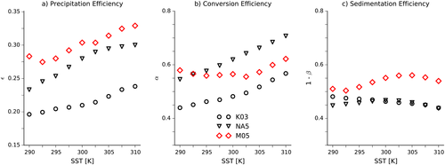
In both sets of simulations with the single-moment scheme the conversion efficiency α increases monotonically with SST (Figure 1b). The sedimentation efficiency 1 − β decreases slightly in the K03 simulations (Figure 1c), while it first increases with warming and then decreases with warming in the NA5 simulations, though these changes are small. So the increasing precipitation efficiency in these simulations is due to the increasing conversion efficiency, which wins out over the small changes in the sedimentation efficiency.
The M05 simulations are more complicated. The conversion efficiency α decreases for SSTs between 290 K and 295 K, is stable between 295 K and 302.5 K, and then increases again for the warmest SSTs. The sedimentation efficiency 1 − β increases between 292.5 K and 302.5 K and then decreases slightly. Hence, the precipitation efficiency increases between 292.5 K and 302.5 K because less of the falling precipitation re-evaporates, countering the reduced conversion efficiency, while for warmer SSTs the re-evaporation is relatively constant and so the increasing conversion efficiency causes the precipitation efficiency to increase. The reduction in ε between 290 K and 292.5 K is mostly due to a reduction in the conversion efficiency, though there is also a small reduction in the sedimentation efficiency.
Comparing the three sets of simulations, the conversion efficiency is smallest in the K03 simulations and largest in the NA5 simulations, except for the two coldest simulations in which α is larger in the M05 simulations. The sedimentation efficiency is always larger in the M05 simulations than in the single-moment simulations, and the K03 and NA5 simulations have similar values of β. So the precipitation efficiency is largest in the M05 simulations because the smallest fraction of falling precipitation is re-evaporated, and the precipitation efficiency is lowest in the K03 simulations because cloud condensate is converted into precipitation less efficiently than in the NA5 simulations.
3.2 Changes in Conversion Efficiency
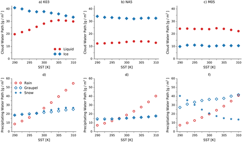
To understand the changes in α, we begin by describing the abundances of the different condensed water phases in the small domain simulations. Comparing panels (a) and (d) of Figure 2 suggests that in the single-moment simulations the increases in α at warmer SSTs are primarily caused by increases in the efficiency with which cloud liquid water is converted into rain, as the mass of rain increases by a factor of more than five from the coldest to the warmest simulation with both parameter settings (Figures 2d and 2e). In the K03 simulations, the mass of cloud liquid water only increases by about 50%, while it is relatively constant in the NA5 simulations (Figures 2a and 2b). In the K03 simulations, the mass of cloud ice decreases by about 20% over the course of the simulations but otherwise changes in the masses of the frozen phases are small.
 (5)
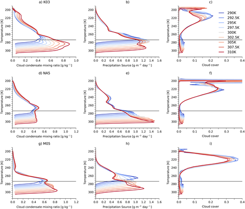
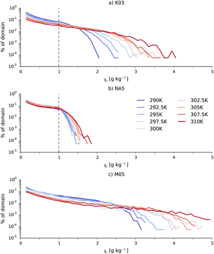
(5)Denser clouds convert condensate into precipitation more efficiently in this scheme, and Figure 3a shows that the cloud condensate density increases at almost all heights as the SST is increased in the K03 simulations. As another way of showing this, probability density functions (PDFs) of qc at the altitudes of maximum time-mean condensation are plotted for these simulations in Figure 4a. The PDFs have a consistent structure across the simulations, decaying exponentially with qc, before reaching a cutoff value after which the probability density decays more rapidly. The slopes of the PDFs weaken, and the cutoff values increase as the underlying SST is increased, and both of these changes result in a rapid increase in the fraction of the domain that is above the qc,0 value for rain (1 g/kg) with surface warming.
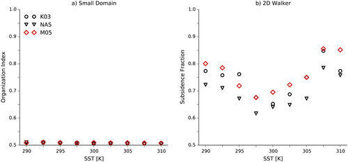
Since both the slope and the cutoff change, it is difficult to say what causes the cloud density to increase. One possibility is that the cloud densities increase because the convection becomes more organized, with fewer scattered, thin clouds and more deep convective towers (Becker et al., 2015); however, measures of convective organization, such as the subsidence fraction (the fraction of the domain with ω500> 0; Coppin & Bony, 2015) and the index of convective organization (Tompkins & Semie, 2017) have little variation across the simulations (Figure 5a). As mentioned above, Muller and Held (2012) found this domain size to be too small for convection to aggregate.
Alternatively, we note that the mean cloud density increases by between 2% and 6% K−1 in the K03 simulations (circles in Figure 6a), which is in the range of values that would be expected for clouds formed by undilute ascent along a moist adiabat (Betts, 1987). Although the clouds here are unlikely to be formed by undilute ascent, the increased availability of water for warmer SSTs probably does contribute to the increasing cloud density, and in Appendix Appendix A we provide an argument for why the density of clouds formed by entraining plumes will also increase with warming, though at a slower rate than clouds formed by undilute plumes.
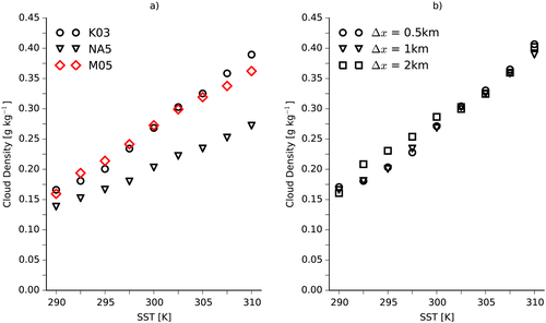
The cloud condensate mixing ratios are smaller in the NA5 simulations (Figure 3d) and have a different vertical profile, being roughly uniform between the subcloud layer and about 263 K and then decreasing at colder temperatures. The density increases more slowly as the SST is increased than in the K03 simulations (triangles in Figure 6a), while the slopes of the PDFs do not change with SST, though the cutoff values again increase in warmer climates (Figure 4b).
There is more liquid cloud water than cloud ice in the M05 simulations because the microphysics maintains more supercooled water (not shown), but the ratio of these stays constant across the simulations (Figure 2c). The mass of graupel increases slightly as the SST is increased, and the mass of rain again increases rapidly, but the mass of snow decreases substantially (Figure 2f). This decrease in the mass of snow is responsible for the nonmonotonicity in α, as the mass of cloud ice stays fixed.
The profiles of qc and of the precipitation source are similar in the M05 simulations to those in the NA5 simulations (Figures 3g and 3h), and the increase in liquid precipitation is again due to an increase in the range of altitudes with thick liquid clouds. However, in the M05 simulations the peak in the precipitation source is higher in the atmosphere than in the NA5 simulations, and in the coldest simulations it is above the freezing line. So the amount of snow decreases as the SST increases because the peak moves to warmer temperatures. That the peak is at colder temperatures in the M05 simulations despite the similar qc profiles implies that precipitation tends to form at colder temperatures in the Morrison scheme than in the single-moment scheme. The mass of cloud ice is roughly constant, as a decrease in the coverage of anvil clouds with surface warming is offset by an increase in their density (Figure 3i), but these clouds form little snow because their densities are still low.
3.3 Changes in Precipitation Evaporation
A number of factors influence the re-evaporation of falling precipitation, and the roles these factors play are often not straightforward. For example, when hydrometeors fall faster, there is less time for them to be re-evaporated, but this also increases the “ventilation factor” (Lin et al., 1983), which promotes their evaporation. So faster fall speeds act to both reduce and enhance re-evaporation.
 (6)
(6) (7)
(7) (8)
(8)
The scaling works well for the three sets of simulations, though the slopes differ (Figure 7). The spread around the scaling is largest for the M05 simulations, which likely reflects differences in the microphysics controlling how rain and snow are evaporated in the double-moment scheme that are not accounted for in our scaling. The slope for these simulations is also smaller, which predominantly reflects differences in the parameterizations of how snow and rain are re-evaporated in this scheme. These are not captured by our scaling, and partly explain why the sedimentation efficiencies are greater in this scheme (Figure 1c).
Figure 8 shows how the terms that go into equation 6 vary with SST. The two sets of single-moment simulations are very similar: The saturation deficit decreases as the SST increases (Figure 8a), while the heights and the fall speeds increase as the SST increases (Figures 8b and 8c, respectively), but the heights increase faster than the speeds, so the total fall time increases with warming in both sets of simulations (Figure 8d). The anticorrelation between the saturation deficit and the precipitation efficiency is surprising, given the lower bound on ε given by equation 2.
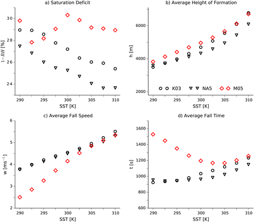
 . (c) Average precipitation fall speeds (w) for the same simulations. (d) Average fall time (t) for the same simulations. SST = sea surface temperature.
The saturation deficit changes nonmonotonically in the M05 simulations, decreasing from 290 K to 292.5 K, then increasing up to 300 K before decreasing again. The formation heights are similar to the single-moment simulations, while the fall speeds are much slower in the colder simulations (2.5 vs. 3.75 m/s at 290 K), because the M05 simulations have more snow (which falls more slowly than rain). But the fall speeds increase rapidly as the amount of snow decreases, and from 302.5 K on the fall speeds are almost the same in the three sets of simulations. The result is that the fall times in the M05 simulations decrease from 290 K to 302.5 K, before increasing again in the warmest simulations.
Returning to Figure 1c, the sedimentation efficiency decreases in the K03 simulations as the SST increases because the fall time increases faster than the saturation deficit decreases, so more precipitation is re-evaporated. In the NA5 simulations the saturation deficit decreases faster than the fall time for the colder simulations, so 1 − β increases at first, and then the fall time increases faster for the warmer simulations and 1 − β decreases. In the M05 simulations the large decreases in the fall speed in the colder simulations causes 1 − β to increase for SSTs up to 302.5 K, and then it decreases in the warmest simulations when the precipitation is dominated by rain.
3.4 Sensitivity to Resolution
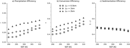
The left panel of Figure 9 compares the precipitation efficiencies in simulations with the K03 microphysics and grid sizes of 0.5, 1, and 2 km. The efficiencies are similar but decrease as the grid size decreases. Comparing the center and right panels of the figure, this is mostly because the conversion efficiency decreases as the grid size decreases, as the re-evaporation is unaffected by changing the grid size. Figure 6b shows that the average cloud density decreases as the grid size decreases, which we believe is the main cause of the reduced conversion efficiency. We have not explored the reasons for the reduced cloud density when using finer grids, but hypothesize that the rate of entrainment of environmental air into convecting plumes increases as the grid size decreases, reducing the cloud condensate mixing ratios. Using equation 6 shows that the primary cause of the reduced re-evaporation at finer grid sizes is reductions in the saturation deficit for a given SST (not shown). Reduced saturation deficit is also consistent with greater entrainment rates, according to the Romps (2014) model of tropospheric relative humidity.
4 The 2-D Mock-Walker Simulations
The precipitation efficiencies for the 2-D mock-Walker simulations are shown in the left panel of Figure 10. These have a similar range of values to the small domain simulations but do not increase monotonically with SST. Instead, the precipitation efficiencies increase with warming up to 300 K and then decrease.
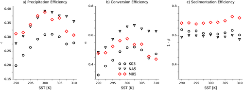
This progression is mostly due to the conversion efficiency (middle panel of Figure 10), which follows the same pattern as ε, increasing from 290 K to 300 K, before decreasing. The changes in 1 − β are small compared to these large changes. Both α and β are smaller than in the corresponding small domain simulations, which is why the values of ε are comparable to those in the small domain simulations, and ε is again smallest in the K03 simulations, though it is now comparable in the NA5 and M05 simulations. From equation 6 it follows that the sedimentation efficiency is larger in these simulations than in the small domain simulations because the relative humidity in the precipitating regions is higher and hence the saturation deficit is lower.
The changes in the conversion efficiency α reflect substantial changes in the organization of convection. For instance, the subsidence fraction decreases by ∼15% when going from 290 K to 297.5 K with all three schemes and increases at warmer SSTs (right panel of Figure 5; as in Cronin & Wing, 2017, the subsidence fraction is calculated in the 2-D Walker simulations by coarse-graining the data into 96-km blocks). This progression with mean SST is similar to what was seen by Coppin and Bony (2015) and by Becker et al. (2015) in simulations of global RCE with uniform SSTs. The top panels of Figure 11 show how the cloud distributions in the K03 simulations are affected by these changes. In the coldest and warmest simulations, the clouds have a bimodal distribution, with narrow regions of deep convection over the warmest SSTs and low clouds decks outside these regions (Figures 11a and 11c). In the 300 K case the strongest convection is still over the warmer SSTs, but it is less intense than in the other simulations and the low cloud decks are less well defined, with evidence of convective activity even over the colder SSTs. (The corresponding NA5 and M05 simulations are very similar.)
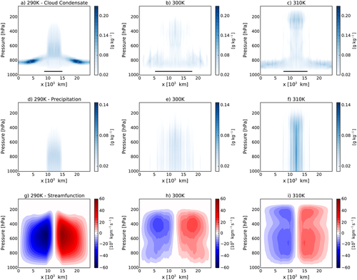
 , where u is the horizontal velocity.
Although the low clouds have large cloud condensate mixing ratios, especially in the 290K case, they have small precipitation efficiencies. The reason for this can be seen from Figure 12, which shows profiles of the “regional” precipitation efficiency (top panel), conversion efficiency (middle panel), and sedimentation efficiency (bottom panel) for the 290 K, the 300 K, and the 310 K mock-Walker simulations with the K03 simulations. These profiles were calculated by averaging the efficiencies over 192-km blocks (note that the domain-average efficiencies are not equal to the average of the regional efficiencies, as these must first be weighted by the local condensation and precipitation). In the 290 K case, the precipitation efficiency is large (>0.4) in the convecting region and small (<0.1) in the subsidence region, reflecting differences in the conversion efficiency, though the sedimentation efficiency is also small over the coldest SSTs. The small conversion efficiency of the low clouds can also be seen by comparing Figures 11a and 11d, as the low clouds have large cloud condensate mixing ratios, but little precipitation.
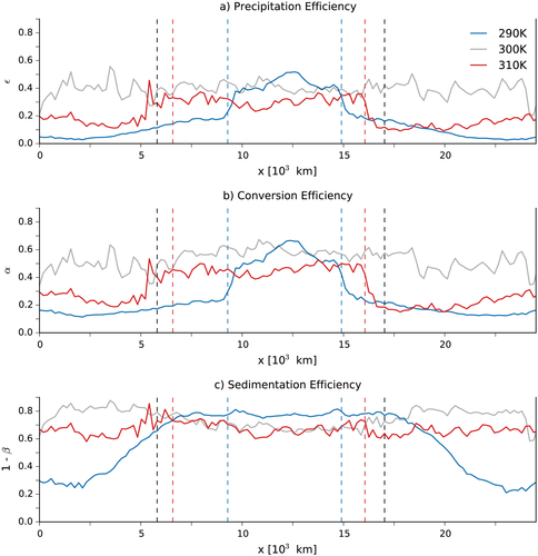
The efficiencies are fairly uniform across the domain in the 300 K case, while in the 310 K case the precipitation efficiency is large in the region of ascent and small in the region of subsidence. In this case the small precipitation efficiency of the low clouds is entirely due to their conversion efficiency, as the sedimentation efficiency is large everywhere. Interestingly, the precipitation efficiency of the deep convection is relatively constant across the simulations, though it is slightly smaller in the 310 K case than in the other two cases (though we note that the values are sensitive to the averaging period).
To understand the differences in conversion efficiency between the low and high clouds, Figure 13 shows PDFs of qc for the 290 K simulation with the K03 scheme for a region of low cloud cover (solid line) and for the center of the domain (dashed line). The PDFs are estimated for the altitudes of maximum time-mean qc at each location. In the low cloud region there is a very sharp cutoff near qc,0, and there are no extreme events during which substantial amounts of precipitation are formed. Conversely, in the region of deep convection the average cloud density is lower, but the distribution is broader and there are periods during which the clouds become very dense and large amounts of precipitation are formed.
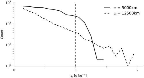
So α increases when going from 290 K to 300 K because of the erosion of the low cloud decks and then decreases as the low clouds reform with surface warming from 300 K to 310 K. This progression is associated with changes in the large-scale circulation, which goes from a single, large overturning cell in the coldest simulations to a double-cell structure in the warmest cases (bottom panels of Figure 11). We are actively investigating the reasons for these changes in the circulation, though we note that Becker et al. (2015) attribute the emergence of a double cell in their global RCE simulations to a strong relative humidity gradient at the top of the boundary layer in the area of subsidence.
There are large changes in the degree of convective aggregation as part of this transition to a double-cell overturning structure, as the convection first becomes less aggregated with surface warming, and then becomes more aggregated with warming for SSTs above 302.5 K. Associated with these changes in aggregation are changes in the large-scale overturning circulation, which affect the stability of the boundary layer over the cold pool. In the 290 K case strong subsidence creates a stronger inversion and hence more low cloud cover over the colder SSTs. In the intermediate cases the subsidence is weaker, leading to a weaker inversion over the cold part of the domain and more convection there. There is strong subsidence over the coldest SSTs in the warmest cases, and the low cloud decks return.
5 Summary and Conclusion
We have investigated how the precipitation efficiency, ε, varies in CRM simulations of RCE as the mean underlying SST is varied from 290 K to 310 K. We have considered three different microphysics schemes and two setups: a small, doubly periodic domain and a wide 2-D domain with a sinusoidal SST profile, whose gradient approximately matches the zonal SST gradient in the equatorial Pacific. In the small domain simulations the precipitation efficiency generally increases with warming because clouds become denser in warmer climates and so cloud condensate is converted more efficiently into precipitation. Changes in the re-evaporation of precipitation are small, though the sedimentation efficiency does tend to increase in warmer climates. In the double-moment simulations there is some added complexity because of large reductions in the amount of snow with warming for SSTs lower than 300 K. In this scheme snow re-evaporates much more readily than rain because of its slower fall speeds, and so the reduction in snow tends to cause the precipitation efficiency to increase, except for when going from 290 K to 292.5 K. We have found that these results are not qualitatively sensitive to the grid size of the simulations, though the precipitation efficiency decreases at finer resolutions because the cloud density decreases.
The precipitation efficiency is not monotonic in the 2-D Walker simulations, as it increases up to about 300 K and then decreases with further warming. This reflects a local minimum in the strength of the large-scale circulation, and consequently in the organization of convection as well, around 300 K. Low cloud fraction in subsidence regions tends to correlate with the strength of the overturning circulation and thus is minimized for surface temperatures near 300 K. Since low clouds have small precipitation efficiencies (≤0.1), the domain-mean precipitation efficiency is largest when the surface temperature is 300 K and smaller for both warmer and colder surfaces.
These results can be summarized as saying that, all else equal, the precipitation efficiency increases with surface warming but may decrease due to changes in the abundances of the different precipitating phases or in the degree of convective organization. With regard to the latter, we have actually found the opposite effect of convective aggregation on precipitation efficiency than what has previously been proposed: Instead of an increase in precipitation efficiency with convective aggregation, increased clustering of convection is associated with an expansion of low cloud decks, which have very small precipitation efficiencies and so the domain-mean precipitation efficiency decreases. We have found no evidence that the precipitation efficiency in the region of strong convection increases with increased clustering.
Our results are a first step towards understanding the sensitivity of the bulk precipitation efficiency of convection to the underlying surface temperature and should be supplemented by future work involving high-resolution process modeling and observational analysis to further constrain how precipitation efficiency is best parameterized in GCMs. Our results also point to the importance of accurately modelling the vertical distributions of the different water phases, especially capturing the temperatures at which precipitation forms. Jiang et al. (2012) have shown that climate models tend to overestimate the amount of liquid water relative to frozen water in the tropical atmosphere, which could be an important source of error in the representation of the precipitation efficiency of tropical clouds.
Returning to the issue of clouds and climate sensitivity, the mock-Walker simulations suggest caution in linking changes in precipitation efficiency and low cloud cover, as any microphysical effects can be overwhelmed by changes in the large-scale tropical circulation. Because of the large difference in efficiency between convecting regions and regions of low clouds, it may also be better to focus on the precipitation efficiency of specific cloud regimes, rather than on the tropical-mean precipitation efficiency. For instance, low clouds in GCMs may have unrealistically large precipitation efficiencies (e.g., GCMs are known to have a “drizzle” problem), and so the GCMs' climates could be overly sensitive to changes in these precipitation efficiencies. On the other hand, the large circulation changes in our mock-Walker simulations may be masking subtle effects related to changes in precipitation efficiency, which would show up in more realistic models whose tropical circulation is not so sensitive. Continuing to untangle the relationship between cloud microphysics and the tropical circulation is a major task for tropical dynamics.
Acknowledgments
We thank Tom Beucler and Kerry Emanuel for helpful comments on earlier drafts of the manuscript and the NSF for support through grant AGS-1623218, “Collaborative Research: Using a Hierarchy of Models to Constrain the Temperature Dependence of Climate Sensitivity”. Simulation data, analysis scripts, and namelist files are available at https://github.com/nicklutsko/Precipitation_Efficiency.
Appendix A: Scaling of Sensitivity of Cloud Liquid Water Content to Temperature
 (A1)
(A1) (A2)
(A2) the saturation mixing ratio along the moist adiabat (i.e., along constant θe,s), Δz = z2−z1, and the angle brackets denoting an average over Δz. This relationship is approximate because it represents a linearization. fu is always less than or equal to the Clausius-Clapeyron scaling
 , and the difference between this scaling and the CC scaling increases as the temperature increases, with a more complex dependence on pressure. For a cloud base at 800 hPa and a temperature of 278.15 K, f is 4.1% K−1 (Betts, 1987).
 (A3)
(A3) is the saturated moist static energy of the plume, ϵ is the entrainment rate, Lv is the latent heat of vaporization,
 is the saturated specific humidity of the plume, and qv,e is the mixing ratio of the environment. Subscript e denotes the environment and moist static energy h = cpT + gz + Lvqv, with cp the specific heat capacity of air and g the gravitational constant. The zero-buoyancy assumption sets the temperature of the plume equal to the environmental temperature T∗=Te, and so
 .
. (A4)
(A4) (A5)
(A5) from equation A4 and rearranging then gives
 (A6)
(A6) and integrating to give
 (A7)
(A7)To illustrate the effects of entrainment on the cloud condensate mixing ratio, Figure A1 plots profiles of qc calculated using equation A7, for plumes originating at 900 hPa with three different temperatures and an environmental RH = 80%. We also follow Singh and O'Gorman in setting
 and perform the calculations using
 = 0 (i.e., undilute ascent), 0.5, and 1.5. Panel (a) of Figure A1 shows that the cloud condensate mixing ratio increases with the cloud-base temperature and decreases significantly with
 . Panel (b) shows the fractional change in the mixing ratio as the cloud-base temperature is increased. As in Betts and Harshvardhan, the fractional change decreases as the cloud-base temperature increases, and again the entrainment has a strong effect, substantially reducing the fractional change. From this we infer that, assuming entrainment rates are not affected by temperature, the fractional change in qc with temperature for a dilute plume will be greater than zero but less than the fractional increase of an undilute plume.
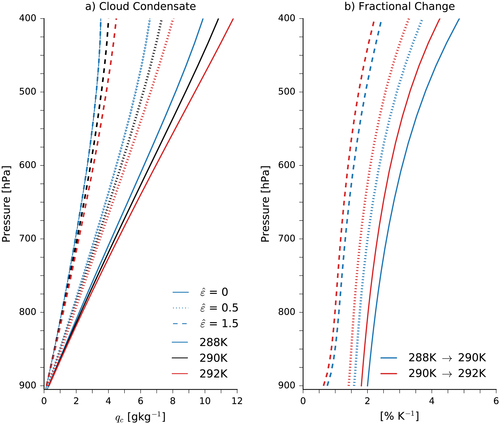
 of 0.5, and the dashed lines include entrainment with
 of 1.5. (b) Fractional change in cloud condensate mixing ratio when increasing the cloud-base temperature from 288 K to 290 K (blue lines) and from 290 K to 292 K (red lines). The solid, dotted, and dashed lines have the same meaning as in panel (a).


